Motivation
Many widely used optimal control tools use pseudospectral collocation as the transcription method for trajectory optimization. For example, GPOPS-II (Patterson, M. A., & Rao, A. V. (2014)), PSOPT (Becerra, V. M. (2010)), and OpenMDAO Dymos (Falck, R., et al. (2021)).
This article shows how to implement Legendre–Gauss–Radau (LGR) pseudospectral collocation in CasADi (Andersson, J. A. E., Gillis, J., Horn, G., et al. (2019)), focusing on the p-method (single interval, raise polynomial degree). The goal is to make the mapping between theory and code explicit. We’ll use a small double-integrator example to set the foundation.
From here, readers can explore hp-adaptive (Darby, C. L., Hager, W. W., & Rao, A. V. (2011)) refinements and other adaptive strategies on top of this tutorial.
Problem Setup
Imagine a simple scenario of driving a car in a straight line. We can only control the acceleration and deceleration, and we have a limit on how hard we can push. Define the state and control
where is position , is velocity , and is acceleration . The state-space dynamics are
The car starts at rest and should arrive at meters, also at rest. We want it fast but without wasting effort, so we use a Bolza objective (time + quadratic control):
Putting it together as an optimal control problem:
import numpy as np
import casadi as ca
from scipy.special import roots_jacobi

A_max = 2.5
L     = 100.0
N     = 20
Time mapping
We need a fixed grid to use LGR. LGR nodes live on . Our problem lives on . So we map time with a simple affine function that sends to and to :
Now we convert both the dynamics and objective. We view . By the chain rule,
The control bound is pointwise and unchanged: . Endpoints move to the ends of :
For the objective, we start with the general form,
Change variables using :
so
For our case we start at . Plugging in,
opti  = ca.Opti()
tf    = opti.variable()
phase = 0.5 * tf
LGR nodes and weights
Our dynamics are continuous in time. To make the problem computable, we discretize by picking a finite set of times (collocation points), enforce the physics only at those points, and interpolate between them with a Lagrange polynomial built on our chosen nodes. We’ll use Left Legendre–Gauss–Radau (LGR) points on . “Left” means we include the left endpoint as a collocation node (good because the initial state is known), and fill the interior with special nodes from orthogonal polynomial theory.
The Gauss–Radau collocation nodes satisfy the Legendre relation
with included as a node. In practice (following Hale, N., & Townsend, A. (2013)), we construct these nodes by taking and attaching it to the roots of the Jacobi polynomial . Those roots give exactly the interior Radau nodes. Conveniently, SciPy exposes these roots and their Gauss–Jacobi weights via roots_jacobi(N-1, 0, 1). The internal algorithm is out of scope of this article, but readers are encouraged to check the SciPy's official documentation about roots_jacobi.
Why do we also need the weights? Because we’ll approximate integrals (for the objective) by a weighted sum on . For Left LGR the Radau weights are:
and they satisfy . Equivalently, take the Gauss–Jacobi weights returned by SciPy for (these integrate on ), and convert interior weights by
We’ll use these inside the cost as
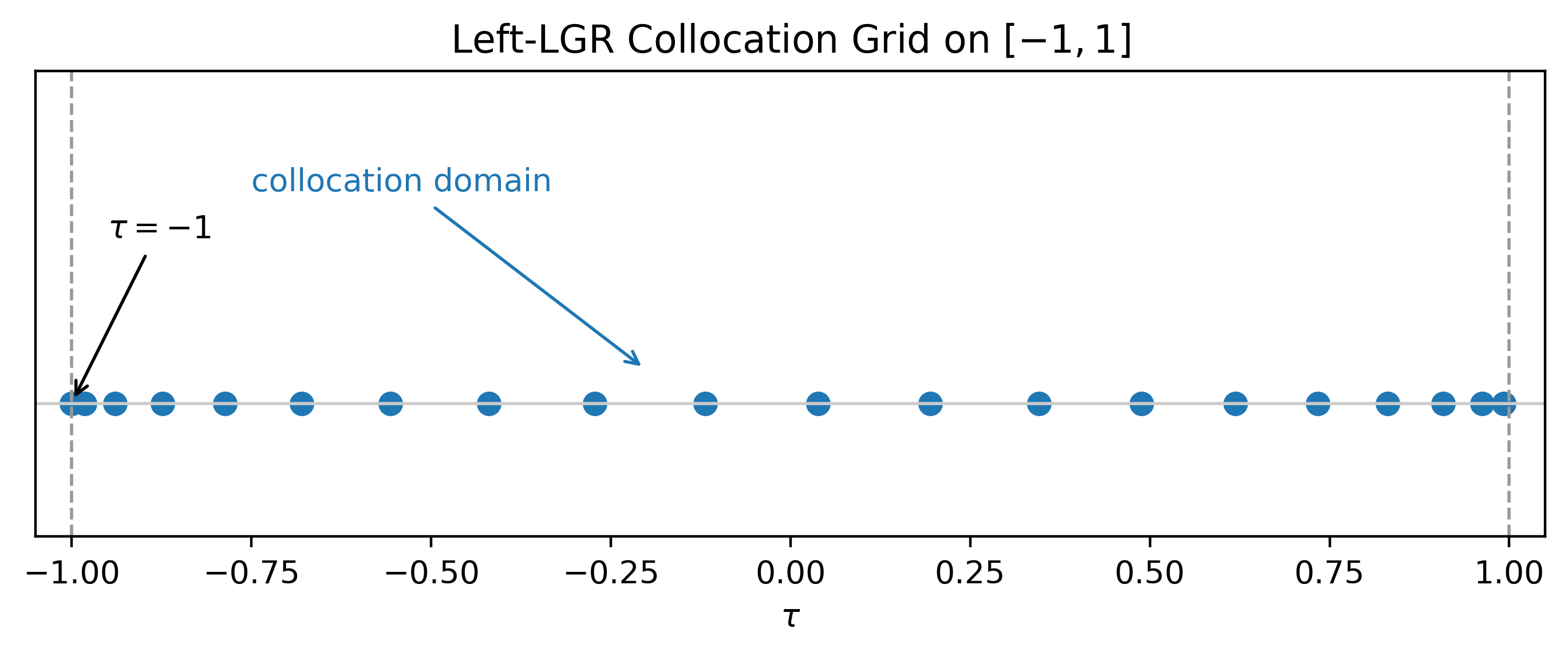 Left LGR collocation nodes distributed across .
def lgr_left_nodes_weights(N):
    if N == 1:
        colloc = np.array([-1.0], dtype=float)
        w_lgr  = np.array([2.0], dtype=float)
    else:
        x, w_gj = roots_jacobi(N-1, 0.0, 1.0)
        x   = np.sort(np.asarray(x, float))
        wgj = np.asarray(w_gj, float)
        colloc = np.concatenate(([-1.0], x))
        w_int  = wgj / (1.0 + x)
        w_lgr  = np.concatenate(([2.0/(N**2)], w_int))
    state = np.concatenate((colloc, [1.0]))
    return colloc, w_lgr, state
Lagrange interpolation and Barycentric
We store the state on the state grid . The classic Lagrange basis is
Given nodal values , the interpolant is
Directly evaluating Lagrange is numerically unstable for moderate , it builds big products, suffers cancellation near nodes, and is slower than it needs to be. The barycentric form evaluates the same polynomial but in a stable way. This isn’t an approximation. Berrut & Trefethen showed that the barycentric and Lagrange forms are mathematically identical. Barycentric is just the robust way to compute it.
We define the first-form barycentric weights as
With these, the barycentric interpolant is
_NUM_EPS = 1e-14

def barycentric_weights(nodes):
    x = np.asarray(nodes, float)
    M = len(x)
    w = np.ones(M, float)
    for j in range(M):
        prod = 1.0
        xj = x[j]
        for m in range(M):
            if m == j:
                continue
            d = xj - x[m]
            if abs(d) < _NUM_EPS:
                d = _NUM_EPS if d == 0 else np.sign(d) * _NUM_EPS
            prod *= d
        w[j] = 1.0 / prod
    return w
Dynamics matching at the collocation nodes
Our model is in state space: . To enforce this at the collocation nodes, we first need from our polynomial interpolant.
First, differentiate the interpolant. We wrote the state on the state grid as
so its derivative is
We evaluate that derivative at each collocation node. Left LGR includes the collocation nodes in the state grid, so for a collocation node we can use the included-node barycentric identity (with first-form barycentric weights on ):
Stacking these coefficients for all gives the -th row of a rectangular matrix , with
To quickly check your implementation, each row of should sums to zero (derivative of a constant).
Finally, match the dynamics via the time map. From the time mapping, , so
Enforcing this at the collocation nodes gives the dynamics-matching equations:
We need to enforce . We get by differentiating the interpolant then we evaluate it at the collocation nodes using the included-node barycentric formula, and we scale it by from the time map (Berrut, J.-P., & Trefethen, L. N. (2004)).
def D_rect(colloc_nodes, state_nodes, w_state):
    C = len(colloc_nodes)
    M = len(state_nodes)
    x = np.asarray(state_nodes, float)
    w = np.asarray(w_state, float)
    D = np.zeros((C, M), float)
    for i in range(C):
        xi = float(colloc_nodes[i])
        jstar = int(np.argmin(np.abs(x - xi)))
        wi = w[jstar]
        s = 0.0
        for j in range(M):
            if j == jstar:
                continue
            d = xi - x[j]
            if abs(d) < _NUM_EPS:
                d = _NUM_EPS if d == 0 else np.sign(d) * _NUM_EPS
            Dij = w[j] / (wi * d)
            D[i, j] = Dij
            s += Dij
        D[i, jstar] = -s
    return D
Discrete OCP on the LGR grid (ready for the solver)
We now write everything on the fixed grid. The decision variables are , the state samples (rows ) at the state grid, and the control samples at the collocation nodes. Using the time map and the derivative matrix , form
Dynamics matching at the nodes:
Bounds and endpoints:
Objective on the LGR grid:
By construction, has rows indexed by collocation nodes () and columns indexed by state nodes (), with entries . We store state samples as columns of : . The derivative of the interpolant at collocation node is
Multiplying on the right by makes each column of produce exactly that sum:
Shapes align naturally: is , is , so is , one column per collocation node. That’s why we use the transpose.
# variables
U  = opti.variable(1, N)        # control at collocation nodes
X  = opti.variable(2, N+1)      # states at state-grid nodes (rows: p, v)

# dynamics matching: X D^T = (tf/2) * [v; U]
Xtau = ca.mtimes(X, ca.DM(D_tau).T)   # 2 x N
F    = ca.vertcat(X[1, 0:N], U)       # 2 x N
opti.subject_to(Xtau == phase * F)

# bounds and endpoints
opti.subject_to(U <=  A_max)
opti.subject_to(U >= -A_max)
opti.subject_to(X[0, 0] == 0)
opti.subject_to(X[1, 0] == 0)
opti.subject_to(X[0, -1] == L)
opti.subject_to(X[1, -1] == 0)
opti.subject_to(tf > 0)

# objective: J = tf + (tf/2) * sum w_i U_i^2
J = tf + phase * ca.mtimes(ca.power(U, 2), ca.DM(w_lgr))
opti.minimize(J)
Assemble the NLP in CasADi
Now we put the pieces together. The decision variables are:
- the final time ,
- the control samples at the collocation nodes,
- the state samples at the state-grid nodes.
We already have:
- Left–LGR nodes and weights on ,
- the state grid ,
- the barycentric weights on ,
- the rectangular derivative matrix ,
- the time map scale .
We enforce the dynamics by matching the interpolant derivative to the scaled model at the collocation nodes:
Add the pointwise control bound , the endpoints , , the positivity , and the cost
# initial guesses
opti.set_initial(tf, 20)
opti.set_initial(X, 0)
opti.set_initial(U, 0)

opti.solver("ipopt")
sol = opti.solve()
Full assembled code
import numpy as np
import casadi as ca
from scipy.special import roots_jacobi
A_max = 2.5
L = 100.0
N = 20
# Left-LGR nodes and weights
def lgr_left_nodes_weights(N):
if N == 1:
colloc = np.array([-1.0], dtype=float)
w_lgr = np.array([2.0], dtype=float)
else:
x, w_gj = roots_jacobi(N-1, 0.0, 1.0) # zeros/weights of P_{N-1}^{(0,1)}
x = np.sort(np.asarray(x, float))
wgj = np.asarray(w_gj, float)
colloc = np.concatenate(([-1.0], x))
w_int = wgj / (1.0 + x) # convert to Left Radau (unit weight)
w_lgr = np.concatenate(([2.0/(N**2)], w_int))
state = np.concatenate((colloc, [1.0]))
return colloc, w_lgr, state
# Barycentric weights
_NUM_EPS = 1e-14
def barycentric_weights(nodes):
x = np.asarray(nodes, float)
M = len(x)
w = np.ones(M, float)
for j in range(M):
prod = 1.0
xj = x[j]
for m in range(M):
if m == j:
continue
d = xj - x[m]
if abs(d) < _NUM_EPS:
d = _NUM_EPS if d == 0 else np.sign(d) * _NUM_EPS
prod *= d
w[j] = 1.0 / prod
return w
# Rectangular derivative matrix D
def D_rect(colloc_nodes, state_nodes, w_state):
C = len(colloc_nodes)
M = len(state_nodes)
x = np.asarray(state_nodes, float)
w = np.asarray(w_state, float)
D = np.zeros((C, M), float)
for i in range(C):
xi = float(colloc_nodes[i])
jstar = int(np.argmin(np.abs(x - xi)))
wi = w[jstar]
s = 0.0
for j in range(M):
if j == jstar:
continue
d = xi - x[j]
if abs(d) < _NUM_EPS:
d = _NUM_EPS if d == 0 else np.sign(d) * _NUM_EPS
Dij = w[j] / (wi * d)
D[i, j] = Dij
s += Dij
D[i, jstar] = -s
return D
# Build nodes/weights and D on tau in [-1,1]
tau_c, w_lgr, tau_s = lgr_left_nodes_weights(N)
bary_w = barycentric_weights(tau_s)
D_tau = D_rect(tau_c, tau_s, bary_w) # shape: N x (N+1)
# CasADi NLP assembly and solve
opti = ca.Opti()
tf = opti.variable() # final time
U = opti.variable(1, N) # control at collocation nodes
X = opti.variable(2, N+1) # states at state nodes (rows: p, v)
phase = 0.5 * tf
# Dynamics matching at collocation nodes: (X D^T) = (tf/2) * [v; U]
Xtau = ca.mtimes(X, ca.DM(D_tau).T) # 2 x N
F = ca.vertcat(X[1, 0:N], U) # 2 x N
opti.subject_to(Xtau == phase * F)
# Path bounds and endpoints
opti.subject_to(U <= A_max)
opti.subject_to(U >= -A_max)
opti.subject_to(X[0, 0] == 0)
opti.subject_to(X[1, 0] == 0)
opti.subject_to(X[0, -1] == L)
opti.subject_to(X[1, -1] == 0)
opti.subject_to(tf > 0)
# Objective: J = tf + (tf/2) * sum_i w_i * U_i^2
J = tf + phase * ca.mtimes(ca.power(U, 2), ca.DM(w_lgr))
opti.minimize(J)
# Neutral initial guesses
opti.set_initial(tf, 20)
opti.set_initial(X, 0)
opti.set_initial(U, 0)
# Solve
opti.solver("ipopt")
sol = opti.solve()
# Report
_tf = float(sol.value(tf))
_X = np.array(sol.value(X))
_U = np.array(sol.value(U)).ravel()
quad_u = float(np.dot(_U**2, w_lgr))
J_val = _tf + 0.5*_tf*quad_u
print(f"tf (s): {_tf:.9f}")
print(f"J = tf + (tf/2) sum w_i U_i^2 = {J_val:.9f}")
print(f"p(0), v(0) = ({_X[0,0]:.6f}, {_X[1,0]:.6f}) p(tf), v(tf) = ({_X[0,-1]:.6f}, {_X[1,-1]:.6f})")
print("max |U|:", float(np.max(np.abs(_U))))
print("sum w (should be 2):", float(np.sum(w_lgr)))
print("max row-sum |D| (should be ~0):", float(np.max(np.abs(D_tau.sum(axis=1)))))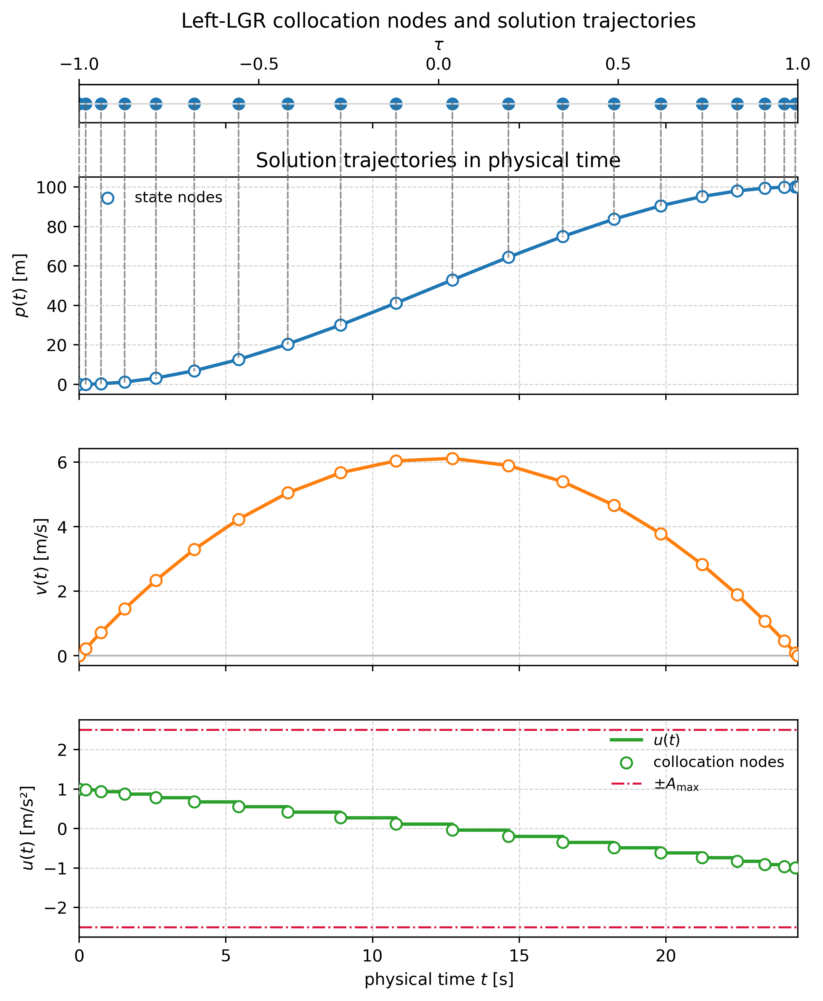 Position, velocity, and control trajectories produced by the full CasADi transcription.
Comparison with the analytical solution
Now we compare to the closed-form solution available for the pure time-optimal problem. To the best of my knowledge, no general closed-form solution exists for objectives that combine final time and control effort. Therefore, let's consider the pure minimum time optimization problem where we only minimize the final time without minimizing the control effort.
J = tf
opti.minimize(J)
We adapt the 1D bang–bang relations from (LaValle, A. J., Sakcak, B., & LaValle, S. M. (2023)) to this article's notation .
We then set
From (35):
Insert (37) into (34) with (36):
Hence
And
Assume , , so the analytic reference is .
| N | [s] | [s] | rel. err [%] |
|---|---|---|---|
| 10 | 12.7174106 | 0.0683000 | 0.5399589 |
| 20 | 12.6657245 | 0.0166139 | 0.1313443 |
| 30 | 12.6564367 | 0.0073260 | 0.0579173 |
| 40 | 12.6532163 | 0.0041057 | 0.0324581 |
| 50 | 12.6517326 | 0.0026220 | 0.0207288 |
References
Patterson, M. A., & Rao, A. V. (2014). GPOPS-II: A MATLAB software for solving multiple-phase optimal control problems using hp-adaptive Gaussian quadrature collocation methods and sparse nonlinear programming. ACM Transactions on Mathematical Software, 41(1), Article 1. https://doi.org/10.1145/2558904
Becerra, V. M. (2010). Solving complex optimal control problems at no cost with PSOPT. In 2010 IEEE International Symposium on Computer-Aided Control System Design (CACSD) (pp. 1391–1396). IEEE. https://doi.org/10.1109/CACSD.2010.5612676
Falck, R., et al. (2021). Dymos: A Python package for optimal control of multidisciplinary systems. Journal of Open Source Software, 6(59), 2809. https://doi.org/10.21105/joss.02809
Andersson, J. A. E., Gillis, J., Horn, G., et al. (2019). CasADi: A software framework for nonlinear optimization and optimal control. Mathematical Programming Computation, 11, 1–36. https://doi.org/10.1007/s12532-018-0139-4
Darby, C. L., Hager, W. W., & Rao, A. V. (2011). An hp-adaptive pseudospectral method for solving optimal control problems. Optimal Control Applications and Methods, 32, 476–502. https://doi.org/10.1002/oca.957
Virtanen, P., Gommers, R., Oliphant, T. E., Haberland, M., Reddy, T., Cournapeau, D., Burovski, E., Peterson, P., Weckesser, W., Bright, J., van der Walt, S. J., Brett, M., Wilson, J., Millman, K. J., Mayorov, N., Nelson, A. R. J., Jones, E., Kern, R., Larson, E., … SciPy 1.0 Contributors. (2020). SciPy 1.0: Fundamental algorithms for scientific computing in Python. Nature Methods, 17(3), 261–272. https://doi.org/10.1038/s41592-019-0686-2
Berrut, J.-P., & Trefethen, L. N. (2004). Barycentric Lagrange interpolation. SIAM Review, 46(3), 501–517. https://doi.org/10.1137/S0036144502417715
Hale, N., & Townsend, A. (2013). Fast and accurate computation of Gauss–Legendre and Gauss–Jacobi quadrature nodes and weights. SIAM Journal on Scientific Computing, 35(2), A652–A674. https://doi.org/10.1137/120889873
LaValle, A. J., Sakcak, B., & LaValle, S. M. (2023). Bang-bang boosting of RRTs. In 2023 IEEE/RSJ International Conference on Intelligent Robots and Systems (IROS) (pp. 2869–2876). IEEE. https://doi.org/10.1109/IROS55552.2023.10341760